The assignments solved during the semester: mapping and path planning will be combined into a single control program in the final stage. The overall goal is to implement a controller that will simultaneously move the robot along the planned path, while mapping obstacles and replanning the path if necessary. Please keep this in mind when implementing a mapping application, as structuring it appropriately will make developing the next parts easier.
The goal of the assignment is to use a laser scanner to create an occupancy grid map of the robot's surroundings.
Before the task, you should recall the formulas for coordinate system transformations (e.g., from the robot's local coordinate system to global coordinates).
Use a logarithmic probability representation to derive the occupancy grid map and a conventional representation to visualize it.
pose topic) and build a map during robot
motion.
(Remark 1: note that the scanner is mounted ahead of robot center)
(Remark 2: robot motion may be executed from another, independant script)
nav_msgs/OccupancyGrid message and verify the results in rviz
Note that there are two approaches with giving different results: looking at beams first and then cells along the beam (easier, but less robust) or firstly cells and then beams passing through (a bit more difficult)
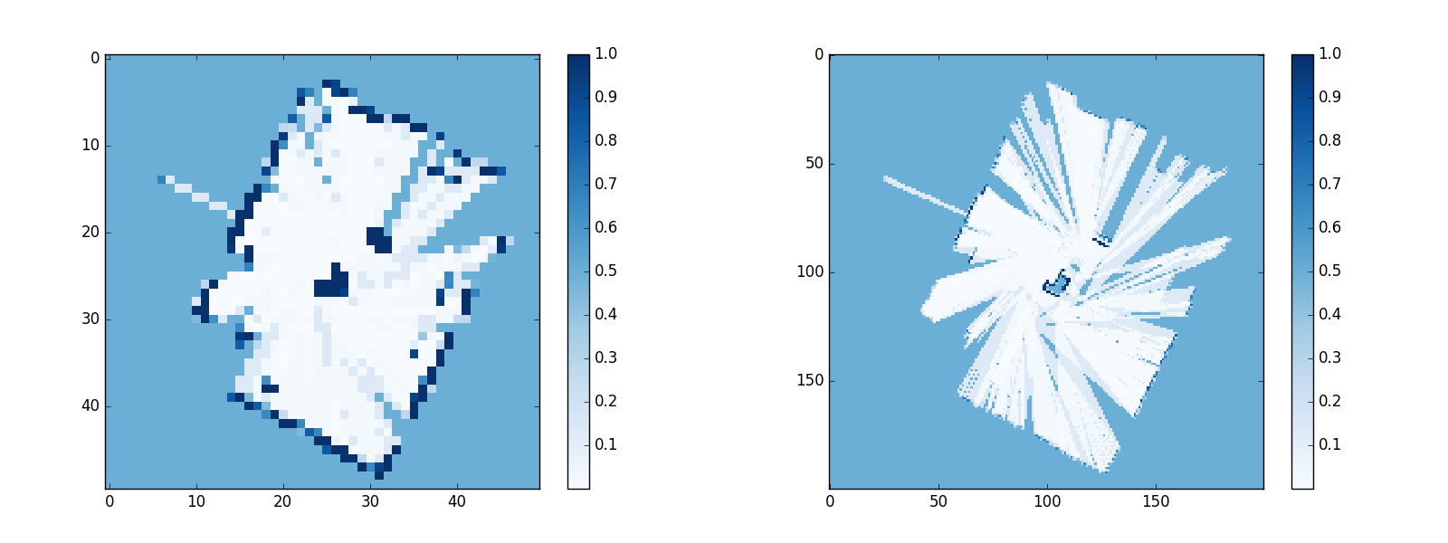
Maps built in laboratory L1.5 with verious resolutions (created by: Beata Berajter, Ada Weiss, Małgorzata Witka-Jeżewska)
import matplotlib as mpl
import matplotlib.pyplot as plt
import numpy as np

f = np.array([[1,2,3], [4,5,6], [7,8,9]]);

plt.imshow(f, interpolation="nearest",cmap='Blues')
plt.colorbar()
plt.show()